Compilation

In this section, you will learn how to:

• understand how compilation chooses the physical scale of an implementation,
• distinguish drive-limited and interaction-limited compilation,
• see why time must be rescaled together with the Hamiltonian

This section describes how QoolQit's compilation maps an abstract programs onto actual hardware.

This page assumes the knowledge of the QoolQit Model page where we introduce the main idea of compilation at a high level: the compiler translates a program, defined in dimensionless units, to the physical scale used to realize it on hardware.

Compilation

From dimensionless programs to physical hardware

A QoolQit program is specified in terms of dimensionless quantities ($\tilde{J}_{ij}$, $\tilde{\Omega}(t)$, $\tilde{\delta}(t)$, $\tilde t$). Once the device, and therefore $J_{\text{max}}$ and $r_{\text{min}}$ are fixed, the conversion to physical units is completely determined:

$$\Omega(t) = J_{\text{max}}\,\tilde{\Omega}(t), \qquad \delta(t) = J_{\text{max}}\,\tilde{\delta}(t), \qquad \Delta(t) = J_{\text{max}}\,\tilde{\Delta}(t), \qquad r_{ij} = r_{\text{min}}\,\tilde r_{ij}, \qquad t = \tilde t/J_{\text{max}}.$$

Thus, a given dimensionless program corresponds to one and only one set of physical parameters on a given device.

In the following step, QoolQit adjusts the dimensionless program so that the resulting physical parameters satisfy the device's operational constraints.

Energy scale maximization

We will now discuss the compilation strategy that QoolQit uses to rescale the compiled program so that it can both run on a physical QPU and fully exploit its capabilities.

As discussed, the user specifies a dimensionless program by providing a register (which determines the values $\tilde J_{ij}$) and a time-dependent drive (amplitude, detuning and phase, which determines $\tilde \Omega(t)$, $\tilde\delta(t)$, $\tilde\Delta(t)$ and $\phi$). Over all these parameters, two in particular are arguably more important since they set the energy scales of the interactions and of the drive, and thus their ratio. Respectively, they are the maximum interaction $\max_{i>j}\tilde J_{ij}$ and the maximum driving amplitude $\max_{\tilde t}\tilde\Omega$ in the defined program.

Thus, simplifying, we will represent a program as a point in the $(\tilde J, \tilde\Omega)$ plane. Interestingly, every program also defines a line through the origin in that plane, with slope $\tilde{\Omega}_{\text{max}}/\tilde{J}_{\text{max}}$. All points lying on the same line are ideally physically identical programs, differing only by a global energy scale factor while preserving the fundamental ratio between driving and interaction strengths.

In addition to the upper bound $\tilde J_{ij} \leq 1$ inherent to the adimensionalization, the device imposes a maximum drive amplitude $\tilde\Omega_{\text{max}} = \Omega_{\max}/J_{\text{max}}$. Together these define a device allowed region represented as a shaded green rectangle in the figure below:

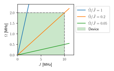
If the user's point lies outside this region, the program cannot be implemented as specified. If it lies strictly inside, the program is feasible but does not exploit the full capability of the device. Compilation resolves both situations by rescaling the program (sliding the point along the line) until it sits exactly on the boundary of the feasible region, maximizing either $\tilde\Omega$ or $\tilde J$, depending on your program.

Why maximize the energy scale?

Higher amplitude guarantees better signal/noise ratio and thus better results, while higher interactions, thus lower distances between atoms help making the register more compact, allowing to put more qubits in your program.

Concretely, compilation rescales all dimensionless parameters by a common factor $\alpha$:

$$\tilde J_{ij}\;\to\;\alpha\,\tilde J_{ij}, \qquad \tilde\Omega\;\to\;\alpha\,\tilde\Omega, \qquad \tilde\delta\;\to\;\alpha\,\tilde\delta,$$

with $\alpha$ chosen as large as possible while keeping the program inside the feasible region. The ratio $\tilde\Omega/\tilde J$ is preserved by construction, so the dimensionless content of the program — the relative balance between drive and interactions — is unchanged.

Drive-limited compilation

When the ratio $\tilde\Omega/\tilde J$ is large, the ray hits the line $\tilde\Omega = \tilde\Omega_{\max}$ before reaching $\tilde J = 1$ (blue line above). The compiled program saturates the drive maximum amplitude:

$$\alpha \,\max_{\tilde t}\tilde\Omega \;=\; \tilde\Omega_{\max} \qquad\Longrightarrow\qquad \alpha \;=\; \frac{\tilde\Omega_{\max}}{\max_{\tilde t}\tilde\Omega}.$$

Atoms are placed further apart than the device minimum: the closest pair sits at a dimensionless distance $\tilde r > 1$, equivalently at a physical distance $r > r_{\min}$.

Interaction-limited compilation

When the ratio $\tilde\Omega/\tilde J$ is small, the ray hits $\tilde J = 1$ before reaching $\tilde\Omega_{\max}$ (red line above). The compiled program saturates the interaction bound:

$$\alpha \,\max_{i<j}\tilde J_{ij} \;=\; 1 \qquad\Longrightarrow\qquad \alpha \;=\; \frac{1}{\max_{i<j}\tilde J_{ij}}.$$

In this case, the closest pair of atoms is placed exactly at the device's minimum spacing $r_{\min}$, and the drive amplitude remains strictly below the device maximum.

Note

Compilation succeeds whenever such an $\alpha$ exists. If multiple values of $\alpha$ would keep the program inside the feasible region, QoolQit chooses the largest one, in order to maximize the physical drive amplitude and minimize the physical runtime.

---

Time scaling

The same rescaling argument that adjusts $\tilde\Omega$ and $\tilde J$ also forces a rescaling of dimensionless time. This follows directly from the Schrödinger equation.

In physical units,

$$i\hbar \frac{d}{dt}|\psi(t)\rangle = H(t)|\psi(t)\rangle.$$

Because $J_{\text{max}}$ is a fixed device constant, the change of variable $\tilde t = J_{\text{max}}t$ rewrites this exactly as

$$i\frac{d}{d\tilde t}|\psi(\tilde t) \rangle = \tilde H(\tilde t)|\psi(\tilde t) \rangle,$$

where $\tilde H = H/J_{\text{max}}$. The conversion $\tilde t = J_{\text{max}} t$ between physical and dimensionless time is therefore fixed by the device, exactly like $\tilde \Omega = \Omega/J_{\text{max}}$.

Now consider what happens during compilation. Compilation multiplies the dimensionless Hamiltonian by a factor $\alpha$:

$$\tilde H(\tilde t)\;\longrightarrow\;\alpha\,\tilde H(\tilde t).$$

For two programs along the same line to represent the same physics,i.e. to generate the same unitary evolution, the dimensionless time variable must be rescaled by the inverse factor:

$$\tilde t\;\longrightarrow\;\tilde t/\alpha.$$

Indeed, with this rescaling,

$$\mathcal{T}\exp\left(-i\int_0^{\tilde t/\alpha}\alpha\,\tilde H(\tilde t')\,d\tilde t'\right) = \mathcal{T}\exp\left(-i\int_0^{\tilde t}\tilde H(s)\,ds\right),$$

the unitary generated by the rescaled program is identical to the unitary generated by the original program.

Compiling time back to physical units

Combining the fixed device conversion $t = \tilde t/J_{\text{max}}$ with the compilation rescaling $\tilde t \to \tilde t/\alpha$, a dimensionless duration $\tilde T$ specified by the user is realized physically in a time

$$T \;=\; \frac{\tilde T/\alpha}{J_{\text{max}}} \;=\; \frac{\tilde T}{\alpha\,J_{\text{max}}}.$$

A larger $\alpha$, that is a program with larger amplitude and interaction, yields a shorter physical runtime. This is consistent with the compilation strategy: by maximizing $\alpha$, QoolQit produces the fastest physical implementation compatible with the device constraints.

Special case: a single atom

The interpretation above relies on interactions being physically present. For a single atom, however, there are no pairwise interaction terms, so $J_0$ is no longer an intrinsic dynamical scale of the problem.

Mathematically, the dimensionless convention still works exactly as before: one may still define

$$\tilde t = \frac{J_0}{\hbar}t$$

and rewrite the Hamiltonian in dimensionless form. But in this case, $J_{\text{max}}$ is only a reference scale introduced by convention. It is not a scale that the dynamics can directly probe, because there is no interaction-driven process in the system.

As a result, saying that time is measured "in units of the interaction" remains mathematically valid, but it is not especially informative physically in the one-atom limit.

For a single atom, time should instead be interpreted through the local dynamics generated by the drive and detuning, namely through quantities such as $\tilde\Omega$ and $\tilde\delta$. For example, when detuning is absent, the natural timescale is the Rabi period set by the drive amplitude. In that regime, the relevant physical question is not how long it takes correlations to spread, but how long it takes the atom to undergo coherent single-particle evolution.

Single-atom programs

For one-atom programs, the dimensionless formulation remains fully consistent and compilable, but the physical interpretation of time is different from the many-body case. Dimensionless time should be understood as a convenient normalized parameterization of the pulse sequence, rather than as an interaction-driven clock.